A PHP Function to Compute the Circumference or Perimeter of an Ellipse or Circle
by Evaluating the Complete Elliptic Integral of the Second Kind Using an Infinite
Power Series Summation Based on Legendre Polynomials.

MathJax equations display requires Java Script to be enabled.
PHP Function by Jay Tanner - 2018


The Complete Elliptic Integral Of The Second Kind

The complete elliptic integral of the second kind may be symbolized as:

$\begin{align*} (Equation~1):~~~~~~~~ \frac{C}{4} = \int_0^{\large\frac{\pi}{2}}{\sqrt{1-\epsilon^2\cdot\sin^2(\phi)}\;\;d\phi} \end{align*}$ =

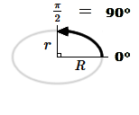
The integral defines the length of the elliptic arc from $0$ to $2\pi$ (or $0$ to $90$°) or only $\frac{1}{4}$ of the full $360$° span of the ellipse.  It is a line integral in the sense that it defines the length of a line, in this case, one quarter of the ellipse circumference. 

Numerically solving the integral is difficult enough as it is, so solving only for the first quarter and then multiplying the result by $4$ seems like the simplest way to go about it.

Notice that the angular arc-span is measured positively counter-clockwise.


The Basic Ellipse

To make use of the integral, we need to adapt it to our purpose, which in this case, is to 'simply' compute the circumference of an ellipse. 

Generally, the idealized equations equate the major radius $(R)$ to unity or ($R = 1$) and this is often left invisible and not clearly indicated.  In the real world, we need to be able to use any units of measure we wish, so we will use $R$ rather than an implied invisible $1$.  Thus, $R$ can be interpreted as any implied units, meters, kilometers, miles, etc.

Given an ellipse with parameters $(R \ge r)$   =  

The elliptic eccentricity $(\epsilon)$, may be found from:

$ (Eq.~2):~~~~~~~~ \begin{align*} \epsilon ~=~ \sqrt{1 - \frac{\Large r^2}{R^2}} \end{align*} $

The eccentricity tells us how much the form of the ellipse deviates from a perfect circle.  Zero means the form is a perfect circle and the greater the value of $\large\epsilon$, within the contstraints $(0 ~\le~ \large\epsilon ~\lt~ 1)$, the 'flatter' the ellipse. 

The symbol $\large(\epsilon)$ (Greek lower-case letter epsilon) is used here for the eccentricity instead of $\large(e)$, so as not to confuse it with Euler's number $\large(e = 2.71828...)$, used as the base of natural logarithms.

To be able to use any desired units of length or distance measure, simply specify the $(R)$ value in any units $($m, km, mi, etc.$)$, so that the resulting circumference $(C)$ will be in the same units as $(R)$.

$\begin{align*} (Eq.~3):~~~~~ \frac{C}{4} ~=~ R \times \int_0^{\large\frac{\pi}{2}}{\sqrt{1-\epsilon^2\cdot\sin^2(\phi)}\;\;d\phi} \end{align*}$  = =

Since the integral equates to $\frac{1}{4}$ the circumference, we must multiply it by $4$ to obtain the full circumference.

$\begin{align*} (Eq.~4):~~~~~ C ~=~ 4R~\times \int_0^{\large\frac{\pi}{2}}{\sqrt{1-\epsilon^2\cdot sin^2(\phi)}\;\;d\phi} \end{align*}$  =  $4$ $\times$ =

The integral above formally defines the problem and the summation equation below provides one of several possible numerical solutions adopted to solve the problem, defined purely in terms of the basic ellipse parameters $(R,~r)$.


Numerical Solution

The numerical computation of the above elliptic integral will involve evaluating the infinite power series summation below until a given precision limit is reached.  This solution is based on Legendre polynomials.

The numerical solution for the quarter-ellipse is expressed by this power series:

$\begin{align*} (Eq.~5):~~~~~ \frac{C}{4} ~=~ \frac{\pi R}{2}\left[ 1 - \sum_{n=1}^\infty \left(\frac{(2n-1)!!~^2}{(2n)!!~^2 \cdot (2n-1)}\right) \cdot {\epsilon ^ {2n}} \right] \end{align*}$

As stated above, since $(Eq.~4)$ only solves for the length of $\frac{1}{4}$ of the ellipse, we have to multply it by $4$ to obtain the full circumference.

Multiplying by $4$ gives the equation:

$ \begin{align*} (Eq.~6):~~~~~~~~ C ~=~ 2\pi{R}\left[ 1 - \sum_{n=1}^\infty \left(\frac{(2n-1)!!~^2}{(2n)!!~^2\cdot(2n-1)}\right) \cdot \epsilon^{2n}\right] ~=~ 2\pi{R}~\left[ 1 - Summation\right] \end{align*} $

Other numerical solutions are possible, but this solution was adopted due to the simplicity of programming it as well as its fast convergence for many practical problems.  $(Eq. 6)$ is numerically evaluated by the PHP function defined below.

If the ellipse is the cross-section of an ellipsoid, then the $(R, ~r)$ parameters respectively represent the equatorial and polar radii, sometimes symbolized as $(a, ~b)$, where $(a \ge b)$.

In the special case of a circle, where ($R = r$), $(\epsilon = 0)$, then $[Summation ~=~ 0]$, and the equation for the circumference reduces to the classical circular circumference equation:

$\begin{align*} (Eq.~7):~~~~~~~~ C ~=~ 2\pi{R}~\left[ 1 - Summation\right] ~=~ 2\pi{R}~[ 1 - 0] ~=~ 2\pi R \end{align*}$

When $(R \ne r)$, then $(0 ~<~ \epsilon ~<~ 1)$ and the form is an ellipse, and computing the circumference will require solving the elliptic integral via a power series summation like the one used here. 

Below is a listing of a PHP function designed to compute the high-precision general circumference of an ellipse.  It is based on $(Eq.~6)$ above and makes use of arbitrary-precision arithmetic to compute the EXACT values of the extremely large integer fractions involved, so it could take several seconds in some extreme cases.

For most practical applications, such as geodesic and meridian computations, the function should converge sufficiently fast and accurately to $16$ decimals  Also, the function could be easily tweaked for higher accuracy, if actually needed. 


The PHP Code

The demonstration program below demonstrates using the function to compute the equatorial and polar meridian circumferences of the Earth according to the WGS-84 Earth ellipsoid model used by the GPS system.  The parameters for any other ellipsoid model could also be used instead.

The function is an implementation of $(Eq. 6)$, above.

Double-Click to select ALL code

Double-Click to select ALL code


Below is the PHP code for only the ellipse circumference function, without all the comments.

Double-Click to select ALL code

Double-Click to select ALL code


What the function above does is delineated by the first few terms of the infinite series worked out
numerically below.  Due to the extremely large numbers, arbitrary-precision is used to maintain
accuracy within the program.

Notice how quickly the numbers become very large in the series.  Although very large at first, the integer
fractions can subsequently be reduced to lowest terms, which reduces the sizes of the numbers used in
the terms, as demonstrated below.

As a visual and mental aid, the first few terms of the summation series are worked out numerically below in $6$ forms.

This is the summation that is evaluated to $16$ decimals by the PHP function defined above.


Summation Series Form 1:

The initial symbolic series, before full numerical expansion, may be written as:

$ \begin{align*} C ~=~ 2\pi R\left[1 - \left[\left(\frac{1!!^2}{2!!^2} \cdot \frac{\epsilon^{2}}{1}\right) + \left(\frac{3!!^2}{4!!^2} \cdot \frac{\epsilon^{4}}{3}\right) + \left(\frac{5!!^2}{6!!^2} \cdot \frac{\epsilon^{6}}{5}\right) + \left(\frac{7!!^2}{8!!^2} \cdot \frac{\epsilon^{8}}{7}\right) + \left(\frac{9!!^2}{10!!^2} \cdot \frac{\epsilon^{10}}{9}\right) + \left(\frac{11!!^2}{12!!^2} \cdot \frac{\epsilon^{12}}{11}\right) + \left(\frac{13!!^2}{14!!^2} \cdot \frac{\epsilon^{14}}{13}\right) + \left(\frac{15!!^2}{16!!^2} \cdot \frac{\epsilon^{16}}{15}\right) + \left(\frac{17!!^2}{18!!^2} \cdot \frac{\epsilon^{18}}{17}\right) + \left(\frac{19!!^2}{20!!^2} \cdot \frac{\epsilon^{20}}{19}\right) + \left(\frac{(2n-1)!!^2}{(2n)!!^2} \cdot \frac{\epsilon^{2n}}{2n-1}\right) + ~ ... ~\right]\right] \end{align*} $


Summation Series Form 2:

Computing the values of the double factorials gives:

$ \begin{align*} C ~=~ 2\pi R\left[1 - \left[\left(\frac{1^2}{2^2} \cdot \frac{\epsilon^{2}}{1}\right) + \left(\frac{3^2}{8^2} \cdot \frac{\epsilon^{4}}{3}\right) + \left(\frac{15^2}{48^2} \cdot \frac{\epsilon^{6}}{5}\right) + \left(\frac{105^2}{384^2} \cdot \frac{\epsilon^{8}}{7}\right) + \left(\frac{945^2}{3840^2} \cdot \frac{\epsilon^{10}}{9}\right) + \left(\frac{10395^2}{46080^2} \cdot \frac{\epsilon^{12}}{11}\right) + \left(\frac{135135^2}{645120^2} \cdot \frac{\epsilon^{14}}{13}\right) + \left(\frac{2027025^2}{10321920^2} \cdot \frac{\epsilon^{16}}{15}\right) + \left(\frac{34459425^2}{185794560^2} \cdot \frac{\epsilon^{18}}{17}\right) + \left(\frac{654729075^2}{3715891200^2} \cdot \frac{\epsilon^{20}}{19}\right) + ~...~ \right] \right] \end{align*} $


Summation Series Form 3:

Computing the integer values in full gives the series in the form:

$ \begin{align*} C ~=~ 2\pi R\left[1 - \left[\left(\frac{1}{4} \cdot \frac{\epsilon^{2}}{1}\right) + \left(\frac{9}{64} \cdot \frac{\epsilon^{4}}{3}\right) + \left(\frac{225}{2304} \cdot \frac{\epsilon^{6}}{5}\right) + \left(\frac{11025}{147456} \cdot \frac{\epsilon^{8}}{7}\right) + \left(\frac{893025}{14745600} \cdot \frac{\epsilon^{10}}{9}\right) + \left(\frac{108056025}{2123366400} \cdot \frac{\epsilon^{12}}{11}\right) + \left(\frac{18261468225}{416179814400} \cdot \frac{\epsilon^{14}}{13}\right) + \left(\frac{4108830350625}{106542032486400} \cdot \frac{\epsilon^{16}}{15}\right) + \left(\frac{1187451971330625}{34519618525593600} \cdot \frac{\epsilon^{18}}{17}\right) + \left(\frac{428670161650355625}{13807847410237440000} \cdot \frac{\epsilon^{20}}{19}\right) + ~ ... ~ \right]\right] \end{align*} $


Summation Series Form 4:

Combining the three integer values in the numerators and denominators of each term in the

series into integer fractions of the form $\left(\frac{Y}{X}\right)$, separate from the powers of $(\epsilon)$, gives:

$ \begin{align*} C ~=~ 2\pi R\left[1 - \left[\left(\frac{1}{4}\right)\cdot{\epsilon^{2}} + \left(\frac{9}{192}\right)\cdot{\epsilon^{4}} + \left(\frac{225}{11520}\right)\cdot{\epsilon^{6}} + \left(\frac{11025}{1032192}\right)\cdot{\epsilon^{8}} + \left(\frac{893025}{132710400}\right)\cdot{\epsilon^{10}} + \left(\frac{108056025}{23357030400}\right)\cdot{\epsilon^{12}} + \left(\frac{18261468225}{5410337587200}\right)\cdot{\epsilon^{14}} + \left(\frac{4108830350625}{1598130487296000}\right)\cdot{\epsilon^{16}} + \left(\frac{1187451971330625}{586833514935091200}\right)\cdot{\epsilon^{18}} + \left(\frac{428670161650355625}{262349100794511360000}\right)\cdot{\epsilon^{20}} + ~ ... ~ \right]\right] \end{align*} $


Summation Series Form 5:

Reducing all of the integer $\left(\frac{Y}{X}\right)$ fractions to their lowest terms to obtain the series in the smallest possible integer values gives:


$ \begin{align*} C ~=~ 2\pi R\left[1 - \left[\left(\frac{1}{4}\right)\cdot{\epsilon^{2}} + \left(\frac{3}{64}\right)\cdot{\epsilon^{4}} + \left(\frac{5}{256}\right)\cdot{\epsilon^{6}} + \left(\frac{175}{16384}\right)\cdot{\epsilon^{8}} + \left(\frac{441}{65536}\right)\cdot{\epsilon^{10}} + \left(\frac{4851}{1048576}\right)\cdot{\epsilon^{12}} + \left(\frac{14157}{4194304}\right)\cdot{\epsilon^{14}} + \left(\frac{2760615}{1073741824}\right)\cdot{\epsilon^{16}} + \left(\frac{8690825}{4294967296}\right)\cdot{\epsilon^{18}} + \left(\frac{112285459}{68719476736}\right)\cdot{\epsilon^{20}} + ~ ... ~ \right]\right] \end{align*} $

It might be noted that in this final reduced fractions series, the fractional denominators all equate to
even powers of $2$, so the summation series could also be expressed in the somewhat abbreviated
form shown below:
Summation Series Form 6:

Abbreviating the powers of $2$ puts the series into the form:

$ \begin{align*} C = 2\pi R\left[1 - \left[\left(\frac{1}{2^{2}}\right)\cdot{\epsilon^{2}} + \left(\frac{3}{2^{6}}\right)\cdot{\epsilon^{4}} + \left(\frac{5}{2^{8}}\right)\cdot{\epsilon^{6}} + \left(\frac{175}{2^{14}}\right)\cdot{\epsilon^{8}} + \left(\frac{441}{2^{16}}\right)\cdot{\epsilon^{10}} + \left(\frac{4851}{2^{20}}\right)\cdot{\epsilon^{12}} + \left(\frac{14157}{2^{22}}\right)\cdot{\epsilon^{14}} + \left(\frac{2760615}{2^{30}}\right)\cdot{\epsilon^{16}} + \left(\frac{8690825}{2^{32}}\right)\cdot{\epsilon^{18}} + \left(\frac{112285459}{2^{36}}\right)\cdot{\epsilon^{20}} + \left(\frac{370263621}{2^{38}}\right)\cdot{\epsilon^{22}} + \left(\frac{19870814327}{2^{44}}\right)\cdot{\epsilon^{24}} + \left(\frac{67607800225}{2^{46}}\right)\cdot{\epsilon^{26}} + \left(\frac{931331941875}{2^{50}}\right)\cdot{\epsilon^{28}} + \left(\frac{3241035157725}{2^{52}}\right)\cdot{\epsilon^{30}} + \left(\frac{2913690606794775}{2^{62}}\right)\cdot{\epsilon^{32}} + \left(\frac{10313859829588425}{2^{64}}\right)\cdot{\epsilon^{34}} + \left(\frac{147068001273760875}{2^{68}}\right)\cdot{\epsilon^{36}} + \left(\frac{527570807893408125}{2^{70}}\right)\cdot{\epsilon^{38}} + \left(\frac{30451387031607516975}{2^{76}}\right)\cdot{\epsilon^{40}} + \left(\frac{110412172026168752025}{2^{78}}\right)\cdot{\epsilon^{42}} + \left(\frac{1608732721339962891075}{2^{82}}\right)\cdot{\epsilon^{44}} + \left(\frac{5884494925884363316125}{2^{84}}\right)\cdot{\epsilon^{46}} + \left(\frac{1382856307582825379289375}{2^{92}}\right)\cdot{\epsilon^{48}} + \left(\frac{5095548922181194957605489}{2^{94}}\right)\cdot{\epsilon^{50}} + \left(\frac{75347791458762166858320219}{2^{98}}\right)\cdot{\epsilon^{52}} + \left(\frac{279375967507591408803895133}{2^{100}}\right)\cdot{\epsilon^{54}} + \left(\frac{16620019291523039931905190055}{2^{106}}\right)\cdot{\epsilon^{56}} + \left(\frac{61954530890516920554723865425}{2^{108}}\right)\cdot{\epsilon^{58}} + \left(\frac{926013721710259572557939375219}{2^{112}}\right)\cdot{\epsilon^{60}} + \left(\frac{3467974385468495527196694913021}{2^{114}}\right)\cdot{\epsilon^{62}} + \left(\frac{13327425563355428311016898550739703}{2^{126}}\right)\cdot{\epsilon^{64}} + \left(\frac{50115525878733222161261891244517065}{2^{128}}\right)\cdot{\epsilon^{66}} + \left(\frac{755201090663955648831472444186407675}{2^{132}}\right)\cdot{\epsilon^{68}} + \left(\frac{2850036442562830175141140497529602189}{2^{134}}\right)\cdot{\epsilon^{70}} + \left(\frac{172374426322411173185388238239475569431}{2^{140}}\right)\cdot{\epsilon^{72}} + \left(\frac{652605297026338283871342029799270910417}{2^{142}}\right)\cdot{\epsilon^{74}} + \left(\frac{9897545709748482283090298097371213946075}{2^{146}}\right)\cdot{\epsilon^{76}} + \left(\frac{37579438838788616163607147608362104233125}{2^{148}}\right)\cdot{\epsilon^{78}} + \left(\frac{9143829058254046084928891156066667202003975}{2^{156}}\right)\cdot{\epsilon^{80}} + \left(\frac{34807473018303177214431870617293636779074025}{2^{158}}\right)\cdot{\epsilon^{82}} + \left(\frac{530636374381070885289400150022823401509557075}{2^{162}}\right)\cdot{\epsilon^{84}} + \left(\frac{2024683407927774524454687971017316980881517125}{2^{164}}\right)\cdot{\epsilon^{86}} + \left(\frac{123739948773767707506962128476636851848089414375}{2^{170}}\right)\cdot{\epsilon^{88}} + \left(\frac{473144900422362152704398894219555132770250042225}{2^{172}}\right)\cdot{\epsilon^{90}} + \left(\frac{7243857369604368761347687418306572817214092801475}{2^{176}}\right)\cdot{\epsilon^{92}} + \left(\frac{27752270221349829256353770312869409575410985685325}{2^{178}}\right)\cdot{\epsilon^{94}} + \left(\frac{27243478600625082386653951190466803733195117614427375}{2^{188}}\right)\cdot{\epsilon^{96}} + \left(\frac{104560039693777648560189987596897791087627242322760625}{2^{190}}\right)\cdot{\epsilon^{98}} + \left(\frac{1606544097886954814597607121428815180503175052840752451}{2^{194}}\right)\cdot{\epsilon^{100}} + ~...~ \right]\right] \end{align*} $

In all of the final reduced fractions, the numerator is always an odd integer and the denominator is always
an even power of $2$.

When $(\epsilon ~=~ 0)$, then the form is a perfect circle and $(Summation = 0)$.

When $(0 ~<~ \epsilon ~<~ 1)$, then the form is an ellipse and $(0 < Summation < 1)$.

The closer that the eccentricity $\large(\epsilon)$ gets to $1$, the longer the series will take to converge. However, for the
intended geophysical and astronomical applications, the elliptic eccentricities don't tend to be so extreme.

One can see that the integers become very large, while the numerator to denominator ratio diminishes
rather slowly, which translates to the series converging more slowly as the eccentricity, or the elliptical
deviation from a perfect circle, increases. 

For small values of eccentricity $\large(\epsilon)$, sufficient approximation formulas could possibly be derived from
the numbers in first few terms of the series.